
A Tour of pyGAM#
Introduction#
Generalized Additive Models (GAMs) are smooth semi-parametric models of the form:
where X.T = [X_1, X_2, ..., X_N] are independent variables, y is the dependent variable, and g() is the link function that relates our predictor variables to the expected value of the dependent variable.
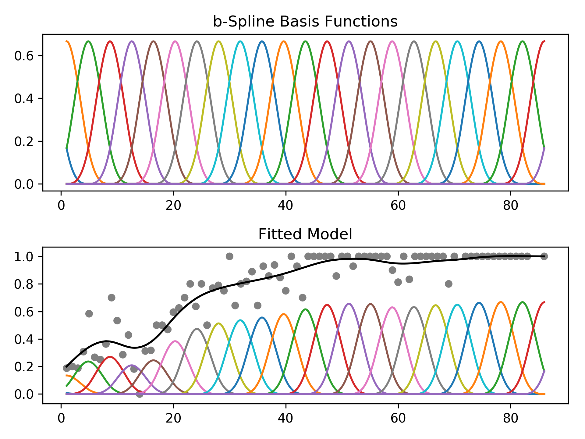
The feature functions f_i() are built using penalized B splines, which allow us to automatically model non-linear relationships without having to manually try out many different transformations on each variable.
GAMs extend generalized linear models by allowing non-linear functions of features while maintaining additivity. Since the model is additive, it is easy to examine the effect of each X_i on Y individually while holding all other predictors constant.
The result is a very flexible model, where it is easy to incorporate prior knowledge and control overfitting.
Generalized Additive Models, in general#
where
So we can see that a GAM has 3 components:
distributionfrom the exponential familylink function\(g(\cdot)\)functional formwith an additive structure \(\beta_0 + f_1(X_1) + f_2(X_2, X_3) + \ldots + f_M(X_N)\)
Distribution:#
Specified via: GAM(distribution='...')
Currently you can choose from the following:
'normal''binomial''poisson''gamma''inv_gauss'
Link function:#
We specify this using: GAM(link='...')
Link functions take the distribution mean to the linear prediction. So far, the following are available:
'identity''logit''inverse''log''inverse-squared'
Functional Form:#
Specified in GAM(terms=...) or more simply GAM(...)
In pyGAM, we specify the functional form using terms:
l()linear terms: for terms like \(X_i\)s()spline termsf()factor termste()tensor productsintercept
With these, we can quickly and compactly build models like:
[12]:
from pygam import GAM, s, te

GAM(s(0, n_splines=200) + te(3, 1) + s(2), distribution="poisson", link="log")
[12]:
GAM(callbacks=['deviance', 'diffs'], distribution='poisson',
   fit_intercept=True, link='log', max_iter=100,
   terms=s(0) + te(3, 1) + s(2), tol=0.0001, verbose=False)
which specifies that we want a:
spline function on feature 0, with 200 basis functions
tensor spline interaction on features 1 and 3
spline function on feature 2
Note:
GAM(..., intercept=True) so models include an intercept by default.
in Practice…#
in pyGAM you can build custom models by specifying these 3 elements, or you can choose from common models:
LinearGAMidentity link and normal distributionLogisticGAMlogit link and binomial distributionPoissonGAMlog link and Poisson distributionGammaGAMlog link and gamma distributionInvGausslog link and inv_gauss distribution
The benefit of the common models is that they have some extra features, apart from reducing boilerplate code.
Terms and Interactions#
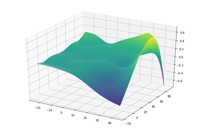
pyGAM can also fit interactions using tensor products via te()
[58]:
from pygam import PoissonGAM, s, te
from pygam.datasets import chicago

X, y = chicago(return_X_y=True)

gam = PoissonGAM(s(0, n_splines=200) + te(3, 1) + s(2)).fit(X, y)
and plot a 3D surface:
[60]:
import matplotlib.pyplot as plt

plt.ion()
plt.rcParams["figure.figsize"] = (12, 8)
[61]:
XX = gam.generate_X_grid(term=1, meshgrid=True)
Z = gam.partial_dependence(term=1, X=XX, meshgrid=True)

ax = plt.axes(projection="3d")
ax.plot_surface(XX[0], XX[1], Z, cmap="viridis")
[61]:
<mpl_toolkits.mplot3d.art3d.Poly3DCollection at 0x7f58f3427cc0>
For simple interactions it is sometimes useful to add a by-variable to a term
[10]:
from pygam import LinearGAM, s
from pygam.datasets import toy_interaction

X, y = toy_interaction(return_X_y=True)

gam = LinearGAM(s(0, by=1)).fit(X, y)
gam.summary()
LinearGAM
=============================================== ==========================================================
Distribution:                        NormalDist Effective DoF:                                     20.8449
Link Function:                     IdentityLink Log Likelihood:                              -2317525.6219
Number of Samples:                        50000 AIC:                                          4635094.9336
                                                AICc:                                         4635094.9536
                                                GCV:                                                  0.01
                                                Scale:                                                0.01
                                                Pseudo R-Squared:                                   0.9976
==========================================================================================================
Feature Function                  Lambda               Rank         EDoF         P > x        Sig. Code
================================= ==================== ============ ============ ============ ============
s(0)                              [0.6]                20           19.8         1.11e-16     ***
intercept                                              1            1.0          1.79e-01
==========================================================================================================
Significance codes:  0 '***' 0.001 '**' 0.01 '*' 0.05 '.' 0.1 ' ' 1

WARNING: Fitting splines and a linear function to a feature introduces a model identifiability problem
         which can cause p-values to appear significant when they are not.

WARNING: p-values calculated in this manner behave correctly for un-penalized models or models with
         known smoothing parameters, but when smoothing parameters have been estimated, the p-values
         are typically lower than they should be, meaning that the tests reject the null too readily.
Regression#
For regression problems, we can use a linear GAM which models:
[17]:
from pygam import LinearGAM, f, s
from pygam.datasets import wage

X, y = wage(return_X_y=True)

## model
gam = LinearGAM(s(0) + s(1) + f(2))
gam.gridsearch(X, y)


## plotting
plt.figure()
fig, axs = plt.subplots(1, 3)
titles = ["year", "age", "education"]
for i, ax in enumerate(axs):
    XX = gam.generate_X_grid(term=i)
    ax.plot(XX[:, i], gam.partial_dependence(term=i, X=XX))
    ax.plot(
        XX[:, i], gam.partial_dependence(term=i, X=XX, width=0.95)[1], c="r", ls="--"
    )
    if i == 0:
        ax.set_ylim(-30, 30)
    ax.set_title(titles[i])
100% (11 of 11) |########################| Elapsed Time: 0:00:01 Time: 0:00:01
<Figure size 864x576 with 0 Axes>
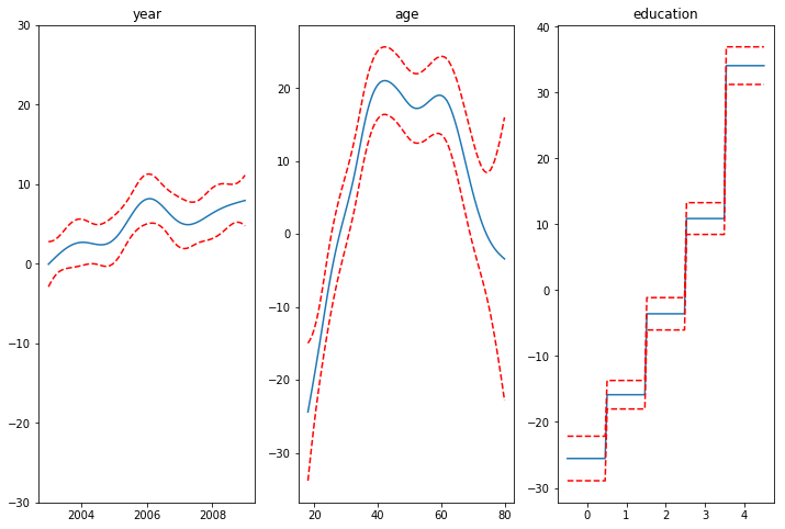
Even though our model allows coefficients, our smoothing penalty reduces us to just 19 effective degrees of freedom:
[4]:
gam.summary()
LinearGAM
=============================================== ==========================================================
Distribution:                        NormalDist Effective DoF:                                     19.2602
Link Function:                     IdentityLink Log Likelihood:                                -24116.7451
Number of Samples:                         3000 AIC:                                            48274.0107
                                                AICc:                                           48274.2999
                                                GCV:                                             1250.3656
                                                Scale:                                           1235.9245
                                                Pseudo R-Squared:                                   0.2945
==========================================================================================================
Feature Function                  Lambda               Rank         EDoF         P > x        Sig. Code
================================= ==================== ============ ============ ============ ============
s(0)                              [15.8489]            20           6.9          5.52e-03     **
s(1)                              [15.8489]            20           8.5          1.11e-16     ***
f(2)                              [15.8489]            5            3.8          1.11e-16     ***
intercept                         0                    1            0.0          1.11e-16     ***
==========================================================================================================
Significance codes:  0 '***' 0.001 '**' 0.01 '*' 0.05 '.' 0.1 ' ' 1

WARNING: Fitting splines and a linear function to a feature introduces a model identifiability problem
         which can cause p-values to appear significant when they are not.

WARNING: p-values calculated in this manner behave correctly for un-penalized models or models with
         known smoothing parameters, but when smoothing parameters have been estimated, the p-values
         are typically lower than they should be, meaning that the tests reject the null too readily.
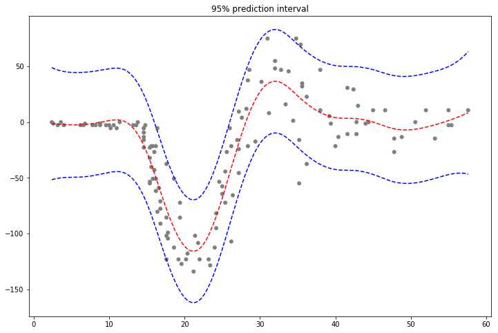
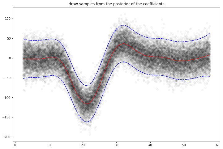
With LinearGAMs, we can also check the prediction intervals:
[56]:
from pygam import LinearGAM
from pygam.datasets import mcycle

X, y = mcycle(return_X_y=True)

gam = LinearGAM(n_splines=25).gridsearch(X, y)
XX = gam.generate_X_grid(term=0, n=500)

plt.plot(XX, gam.predict(XX), "r--")
plt.plot(XX, gam.prediction_intervals(XX, width=0.95), color="b", ls="--")

plt.scatter(X, y, facecolor="gray", edgecolors="none")
plt.title("95% prediction interval");
100% (11 of 11) |########################| Elapsed Time: 0:00:00 Time: 0:00:00
And simulate from the posterior:
[57]:
# continuing last example with the mcycle dataset
for response in gam.sample(X, y, quantity="y", n_draws=50, sample_at_X=XX):
    plt.scatter(XX, response, alpha=0.03, color="k")
plt.plot(XX, gam.predict(XX), "r--")
plt.plot(XX, gam.prediction_intervals(XX, width=0.95), color="b", ls="--")
plt.title("draw samples from the posterior of the coefficients")
100% (11 of 11) |########################| Elapsed Time: 0:00:00 Time:  0:00:00
100% (11 of 11) |########################| Elapsed Time: 0:00:00 Time:  0:00:00
100% (11 of 11) |########################| Elapsed Time: 0:00:00 Time:  0:00:00
100% (11 of 11) |########################| Elapsed Time: 0:00:00 Time:  0:00:00
[57]:
Text(0.5,1,'draw samples from the posterior of the coefficients')
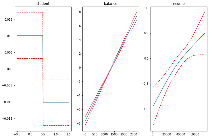
Classification#
For binary classification problems, we can use a logistic GAM which models:
[11]:
from pygam import LogisticGAM, f, s
from pygam.datasets import default

X, y = default(return_X_y=True)

gam = LogisticGAM(f(0) + s(1) + s(2)).gridsearch(X, y)

fig, axs = plt.subplots(1, 3)
titles = ["student", "balance", "income"]

for i, ax in enumerate(axs):
    XX = gam.generate_X_grid(term=i)
    pdep, confi = gam.partial_dependence(term=i, width=0.95)

    ax.plot(XX[:, i], pdep)
    ax.plot(XX[:, i], confi, c="r", ls="--")
    ax.set_title(titles[i])
100% (11 of 11) |########################| Elapsed Time: 0:00:04 Time: 0:00:04
We can then check the accuracy:
[8]:
gam.accuracy(X, y)
[8]:
0.9739
Since the scale of the Binomial distribution is known, our gridsearch minimizes the Un-Biased Risk Estimator (UBRE) objective:
[9]:
gam.summary()
LogisticGAM
=============================================== ==========================================================
Distribution:                      BinomialDist Effective DoF:                                      3.8047
Link Function:                        LogitLink Log Likelihood:                                   -788.877
Number of Samples:                        10000 AIC:                                             1585.3634
                                                AICc:                                             1585.369
                                                UBRE:                                               2.1588
                                                Scale:                                                 1.0
                                                Pseudo R-Squared:                                   0.4598
==========================================================================================================
Feature Function                  Lambda               Rank         EDoF         P > x        Sig. Code
================================= ==================== ============ ============ ============ ============
f(0)                              [1000.]              2            1.7          4.61e-03     **
s(1)                              [1000.]              20           1.2          0.00e+00     ***
s(2)                              [1000.]              20           0.8          3.29e-02     *
intercept                         0                    1            0.0          0.00e+00     ***
==========================================================================================================
Significance codes:  0 '***' 0.001 '**' 0.01 '*' 0.05 '.' 0.1 ' ' 1

WARNING: Fitting splines and a linear function to a feature introduces a model identifiability problem
         which can cause p-values to appear significant when they are not.

WARNING: p-values calculated in this manner behave correctly for un-penalized models or models with
         known smoothing parameters, but when smoothing parameters have been estimated, the p-values
         are typically lower than they should be, meaning that the tests reject the null too readily.
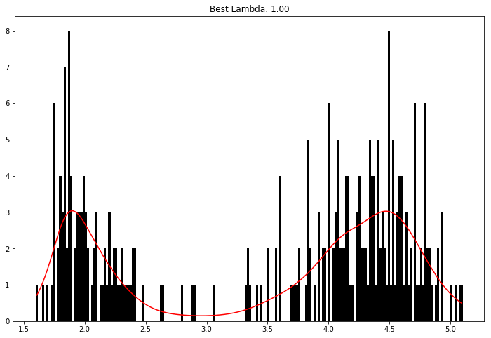
Poisson and Histogram Smoothing#
We can intuitively perform histogram smoothing by modeling the counts in each bin as being distributed Poisson via PoissonGAM.
[10]:
from pygam import PoissonGAM
from pygam.datasets import faithful

X, y = faithful(return_X_y=True)

gam = PoissonGAM().gridsearch(X, y)

plt.hist(faithful(return_X_y=False)["eruptions"], bins=200, color="k")
plt.plot(X, gam.predict(X), color="r")
plt.title(f"Best Lambda: {gam.lam[0][0]:.2f}");
100% (11 of 11) |########################| Elapsed Time: 0:00:00 Time: 0:00:00
Expectiles#
GAMs with a Normal distribution suffer from the limitation of an assumed constant variance. Sometimes this is not an appropriate assumption, because we’d like the variance of our error distribution to vary.
In this case we can resort to modeling the expectiles of a distribution.
Expectiles are intuitively similar to quantiles, but model tail expectations instead of tail mass. Although they are less interpretable, expectiles are much faster to fit, and can also be used to non-parametrically model a distribution.
[52]:
from pygam import ExpectileGAM
from pygam.datasets import mcycle

X, y = mcycle(return_X_y=True)

# lets fit the mean model first by CV
gam50 = ExpectileGAM(expectile=0.5).gridsearch(X, y)

# and copy the smoothing to the other models
lam = gam50.lam

# now fit a few more models
gam95 = ExpectileGAM(expectile=0.95, lam=lam).fit(X, y)
gam75 = ExpectileGAM(expectile=0.75, lam=lam).fit(X, y)
gam25 = ExpectileGAM(expectile=0.25, lam=lam).fit(X, y)
gam05 = ExpectileGAM(expectile=0.05, lam=lam).fit(X, y)
100% (11 of 11) |########################| Elapsed Time: 0:00:00 Time: 0:00:00
[55]:
XX = gam50.generate_X_grid(term=0, n=500)

plt.scatter(X, y, c="k", alpha=0.2)
plt.plot(XX, gam95.predict(XX), label="0.95")
plt.plot(XX, gam75.predict(XX), label="0.75")
plt.plot(XX, gam50.predict(XX), label="0.50")
plt.plot(XX, gam25.predict(XX), label="0.25")
plt.plot(XX, gam05.predict(XX), label="0.05")
plt.legend()
[55]:
<matplotlib.legend.Legend at 0x7f58f816c3c8>
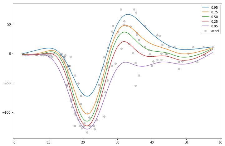
We fit the mean model by cross-validation in order to find the best smoothing parameter lam and then copy it over to the other models.
This practice makes the expectiles less likely to cross.
Custom Models#
It’s also easy to build custom models by using the base GAM class and specifying the distribution and the link function:
[27]:
from pygam import GAM
from pygam.datasets import trees

X, y = trees(return_X_y=True)

gam = GAM(distribution="gamma", link="log")
gam.gridsearch(X, y)

plt.scatter(y, gam.predict(X))
plt.xlabel("true volume")
plt.ylabel("predicted volume")
100% (11 of 11) |########################| Elapsed Time: 0:00:01 Time: 0:00:01
[27]:
Text(0,0.5,'predicted volume')
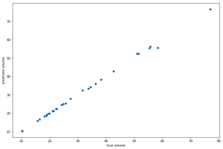
We can check the quality of the fit by looking at the Pseudo R-Squared:
[28]:
gam.summary()
GAM
=============================================== ==========================================================
Distribution:                         GammaDist Effective DoF:                                     25.3616
Link Function:                          LogLink Log Likelihood:                                   -26.1673
Number of Samples:                           31 AIC:                                              105.0579
                                                AICc:                                             501.5549
                                                GCV:                                                0.0088
                                                Scale:                                               0.001
                                                Pseudo R-Squared:                                   0.9993
==========================================================================================================
Feature Function                  Lambda               Rank         EDoF         P > x        Sig. Code
================================= ==================== ============ ============ ============ ============
s(0)                              [0.001]              20                        2.04e-08     ***
s(1)                              [0.001]              20                        7.36e-06     ***
intercept                         0                    1                         4.39e-13     ***
==========================================================================================================
Significance codes:  0 '***' 0.001 '**' 0.01 '*' 0.05 '.' 0.1 ' ' 1

WARNING: Fitting splines and a linear function to a feature introduces a model identifiability problem
         which can cause p-values to appear significant when they are not.

WARNING: p-values calculated in this manner behave correctly for un-penalized models or models with
         known smoothing parameters, but when smoothing parameters have been estimated, the p-values
         are typically lower than they should be, meaning that the tests reject the null too readily.
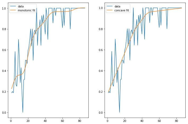
Penalties / Constraints#
With GAMs we can encode prior knowledge and control overfitting by using penalties and constraints.
Available penalties
second derivative smoothing (default on numerical features)
L2 smoothing (default on categorical features)
Available constraints
monotonic increasing/decreasing smoothing
convex/concave smoothing
periodic smoothing [soon…]
We can inject our intuition into our model by using monotonic and concave constraints:
[29]:
from pygam import LinearGAM, s
from pygam.datasets import hepatitis

X, y = hepatitis(return_X_y=True)

gam1 = LinearGAM(s(0, constraints="monotonic_inc")).fit(X, y)
gam2 = LinearGAM(s(0, constraints="concave")).fit(X, y)

fig, ax = plt.subplots(1, 2)
ax[0].plot(X, y, label="data")
ax[0].plot(X, gam1.predict(X), label="monotonic fit")
ax[0].legend()

ax[1].plot(X, y, label="data")
ax[1].plot(X, gam2.predict(X), label="concave fit")
ax[1].legend()
[29]:
<matplotlib.legend.Legend at 0x7fa3970b19e8>
API#
pyGAM is intuitive, modular, and adheres to a familiar API:
[30]:
from pygam import LogisticGAM, f, s
from pygam.datasets import toy_classification

X, y = toy_classification(return_X_y=True, n=5000)

gam = LogisticGAM(s(0) + s(1) + s(2) + s(3) + s(4) + f(5))
gam.fit(X, y)
[30]:
LogisticGAM(callbacks=[Deviance(), Diffs(), Accuracy()],
   fit_intercept=True, lam=[0.6, 0.6, 0.6, 0.6, 0.6, 0.6],
   max_iter=100,
   terms=s(0) + s(1) + s(2) + s(3) + s(4) + f(5) + intercept,
   tol=0.0001, verbose=False)
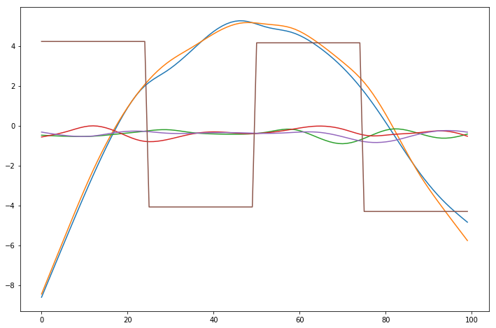
Since GAMs are additive, it is also super easy to visualize each individual feature function, f_i(X_i). These feature functions describe the effect of each X_i on y individually while marginalizing out all other predictors:
[31]:
plt.figure()
for i, term in enumerate(gam.terms):
    if term.isintercept:
        continue
    plt.plot(gam.partial_dependence(term=i))
Current Features#
Models#
pyGAM comes with many models out-of-the-box:
GAM (base class for constructing custom models)
LinearGAM
LogisticGAM
GammaGAM
PoissonGAM
InvGaussGAM
ExpectileGAM
Terms#
l()linear termss()spline termsf()factor termste()tensor productsintercept
Distributions#
Normal
Binomial
Gamma
Poisson
Inverse Gaussian
Link Functions#
Link functions take the distribution mean to the linear prediction. These are the canonical link functions for the above distributions:
Identity
Logit
Inverse
Log
Inverse-squared
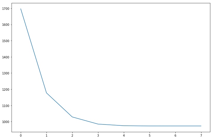
Callbacks#
Callbacks are performed during each optimization iteration. It’s also easy to write your own.
deviance - model deviance
diffs - differences of coefficient norm
accuracy - model accuracy for LogisticGAM
coef - coefficient logging
You can check a callback by inspecting:
[32]:
_ = plt.plot(gam.logs_["deviance"])
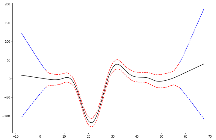
Linear Extrapolation#
[33]:
from pygam import LinearGAM
from pygam.datasets import mcycle

X, y = mcycle()

gam = LinearGAM()
gam.gridsearch(X, y)

XX = gam.generate_X_grid(term=0)

m = X.min()
M = X.max()
XX = np.linspace(m - 10, M + 10, 500)
Xl = np.linspace(m - 10, m, 50)
Xr = np.linspace(M, M + 10, 50)

plt.figure()

plt.plot(XX, gam.predict(XX), "k")
plt.plot(Xl, gam.confidence_intervals(Xl), color="b", ls="--")
plt.plot(Xr, gam.confidence_intervals(Xr), color="b", ls="--")
_ = plt.plot(X, gam.confidence_intervals(X), color="r", ls="--")
100% (11 of 11) |########################| Elapsed Time: 0:00:00 Time: 0:00:00
References#
- Simon N. Wood, 2006Generalized Additive Models: an introduction with R
- Hastie, Tibshirani, FriedmanThe Elements of Statistical Learning
- James, Witten, Hastie and TibshiraniAn Introduction to Statistical Learning
- Paul Eilers & Brian Marx, 1996 Flexible Smoothing with B-splines and Penalties
- Kim Larsen, 2015GAM: The Predictive Modeling Silver Bullet
- Deva Ramanan, 2008UCI Machine Learning: Notes on IRLS
- Paul Eilers, Brian Marx, and Maria Durbán, 2015Twenty years of P-splines
- Keiding, Niels, 1991Age-specific incidence and prevalence: a statistical perspective